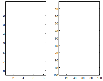
The following function simulates a “random walk,” using a matrix to store the random walk as it progresses

The following function simulates a “random walk,” using a matrix to store the random walk as it progresses. To begin with all elements are initialized to 1. Then, the “middle” element is chosen to be the starting point for the random walk; a 2 is placed in that element. (Note: these numbers will eventually represent colors.) Then, from this starting point another element next to the current one is chosen randomly and the color stored in that element is incremented; this repeats until one of the edges of the matrix is reached. Every time an element is chosen for the next element, it is done randomly by either adding or subtracting one to/from each coordinate (x and y), or leaving it alone. The resulting matrix that is returned is an n by n matrix. 

ranwalk.m

function walkmat = ranwalk(n)

walkmat = ones(n);

x = floor(n/2);

y = floor(n/2);

color = 2;

walkmat(x,y) = color;

while x ~= 1 && x ~= n && y ~= 1 && y ~= n

 x = x + randi([-1 1]);

 y = y + randi([-1 1]);

 color = color + 1;

 walkmat(x,y) = mod(color,65);

end

You are to write a script that will call this function twice (once passing 8

and once passing 100) and display the resulting matrices as images 

side-by-side. Your script must create a custom colormap that has 65 

colors; the first is white and the rest are from the colormap jet. For 

example, the result may look like the Figure. (Note that with the 8 x 8 

matrix the colors are not likely to get out of the blue range, but with 

100 x 00 it cycles through all colors multiple times until an edge is 

reached):

Figure Random walk